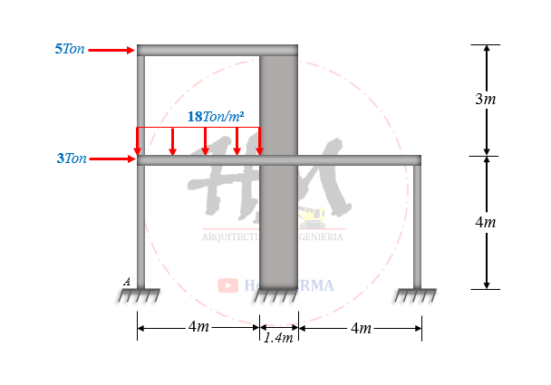
Instrucciones. Analizar el pórtico de dos plantas mostrado en la figura, emplear el Método Matricial de Compatibilidad. Considere una resistencia de concreto de 210kg/cm².

Datos:

• Columnas: 0.25 x 0.25m
• Vigas: 0.25 x 0.50m
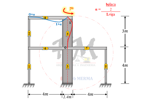
• Espesor de Placa: 0.25m
• μ = 0.15

SOLUCION:

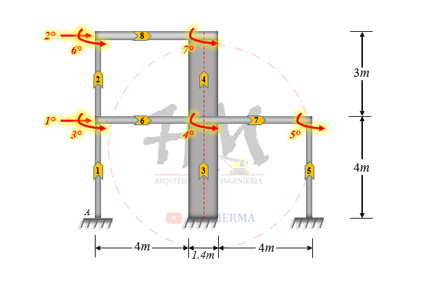
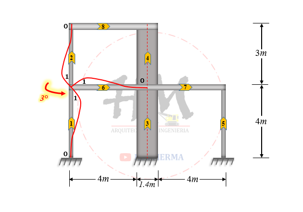
1. Asignar los grados de libertad y orientación de cada elemento.

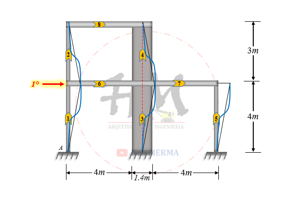
2. Análisis del sistema respecto al 1° GDL.

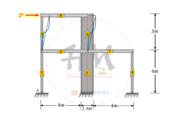
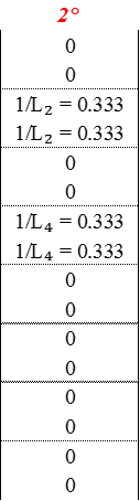
2. Análisis del sistema respecto al 2° GDL.

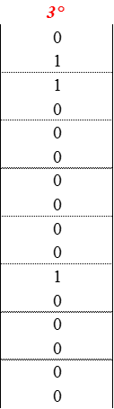
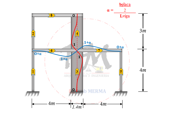
2. Análisis del sistema respecto al 3° GDL.

2. Análisis del sistema respecto al 4° GDL.

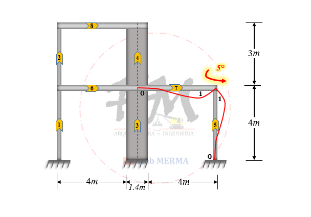
2. Análisis del sistema respecto al 5° GDL.

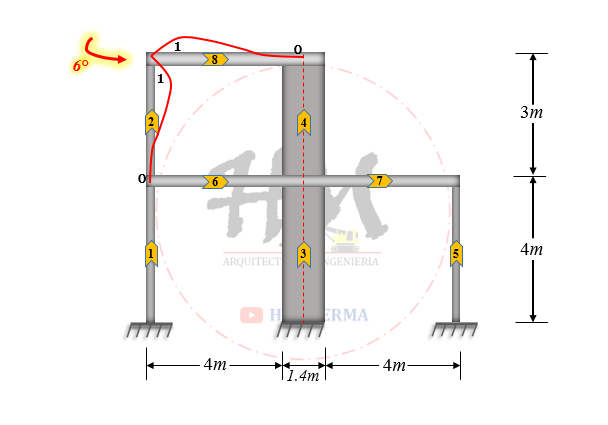
2. Análisis del sistema respecto al 6° GDL.

2. Análisis del sistema respecto al 7° GDL.

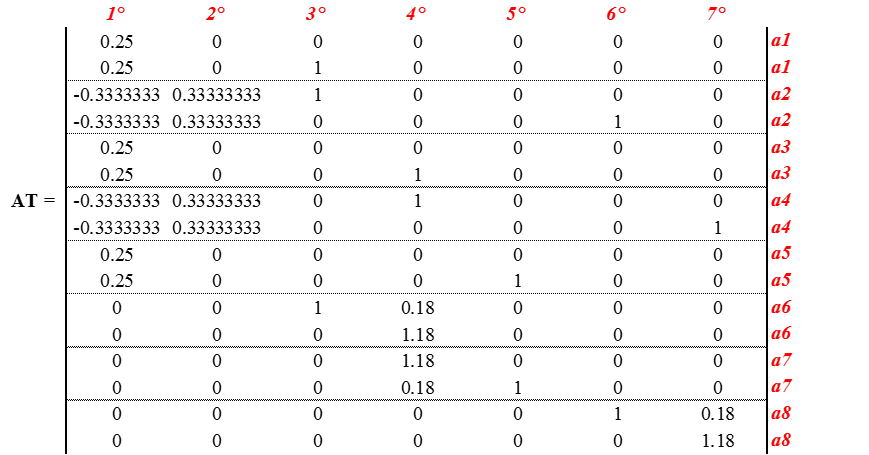
3. Matriz de Compatibilidad.

4. Matriz de Rigidez de cada elemento.

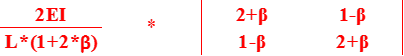
Elemento a Flexión (VIGA – COLUMNA)

Elemento a Corte (PLACA)

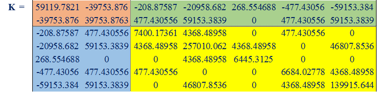
5. Ensamblaje de la Matriz K. K = Σ ɑₑᵀ*Kₑ*ɑₑ

6. Calculo de K Lateral. KLat = Kᴰᴰ – Kᴰᶿ * Kᶿᶿ⁻¹ * Kᶿᴰ